Histogram Equalization and Matching

Code

import cv2
import numpy as np
import matplotlib.pyplot as plt
%matplotlib inline
%config InlineBackend.figure_format = 'retina'

Code

panda = cv2.imread("grey_1.png",0)
lenna = cv2.imread("grey_2.png",0)
campus = cv2.imread("grey_3.png",0)
elon = cv2.imread("grey_4.png",0)

Creating the Histogram of an Image

We have a discrete grayscale image \(\{x\}\) with \(n_i\) as the number of occurences of gray level \(i\). The probability of occurence of a pixel of level \(i\) in the image is \[p_x(i)=p(x=i)=\frac{n_i}{n}, \qquad 0\leq i < L\] where \(L\) is the total number of grey levels in the image (here \(L=256\)), \(n\) is the total number of pixels in the image (here \(n = 512 \times 512\)), and \(p_x(i)\) is the image’s histogram for pixel value \(i\) normalized to \([0,1]\)

Code

def imgToHist(img):
  hist_data = np.zeros((256))
  # counting number of pixels with a particular value between 0-255
  for x_pixel in range(img.shape[0]):
          for y_pixel in range(img.shape[1]):
              pixel_value = int(img[x_pixel, y_pixel])
              hist_data[pixel_value] += 1

  # normalizing
  hist_data/=(img.shape[0]*img.shape[1])

  # returning the hist
  return hist_data

Histogram Equalization

We define the cumulative distribution function corresponsing to \(i\) as \[\text{cdf}_x(i)=\sum\limits_{j=0}^{i}p_x(x=j)\] which is also the image’s accumulated normalized histogram. \ We would like to create a transformation of the form \(y=T(x)\) to produce a new image \(\{y\}\), with a flat histogram. Such as image would have a linearized cumulative distribution function across the value range \[\text{cdf}_y(i)=(i+1)K, \qquad 0 \leq i < L\] for some constant K. The properties of the CDF allow us to perform such a transform: \[y = T(k) = \text{cdf}_x(k)\] where k is in the range \([0, L-1]\). \(T\) maps the levels into \([0,1]\) since we’re using normalized histogram of \(\{x\}\). In order to map the map the values into their original range, the following transformation needs to be applied: \[y' = y \cdot (\text{max}\{x\} - \text{min}\{x\}) + \text{min}\{x\} = y \cdot (L-1)\] \(y\) is a real value while \(y'\) has to be integer. The mapped value \(y'\) should be \(0\) for the range of \(0 < y \leq \frac{1}{L}\). And \(y' = 1\) for \(\frac{1}{L}<y\leq \frac{2}{L}\), \(y' = 2\) for \(\frac{2}{L}<y\leq \frac{3}{L}\), … \(y' = L-1\) for \(\frac{L-1}{L}<y\leq 1\). Then the quantization formula for \(y\) to \(y'\) should be \[y'=\text{ceil}(L \cdot y)-1\] (\(y'=-1\) when \(y=0\), however, it does not happen just because \(y=0\) means that there is no pixel corresponding to that value.)

Code

def equalize(img):
  hist_data = imgToHist(img)
  cdf_hist = np.cumsum(hist_data) # gives the CDF
  equalized_hist = np.ceil(cdf_hist * 256) - 1 # maps back into original range
  enhancedImg = np.zeros_like(img)
  # now we need to replace initial pixel values with final pixel values
  for x_pixel in range(img.shape[0]):
          for y_pixel in range(img.shape[1]):
              pixel_val = int(img[x_pixel, y_pixel])
              enhancedImg[x_pixel, y_pixel] = equalized_hist[pixel_val]
  return enhancedImg

A function is defined to plot an images and their histograms before and after equalization. cmap is explicity defined to be gray since the default color map is virdis

Code

def showEqualizedImg(image, enhanced_image):
  source_histogram = imgToHist(image)
  equalized_histogram = imgToHist(enhanced_image)
  fig, axes = plt.subplots(1, 4, figsize=(16, 4))
  # source image
  axes[0].imshow(image, cmap='gray')
  axes[0].set_title('Source Image')
  axes[0].axis('off')
  # source histogram
  axes[1].bar(np.arange(len(source_histogram)), source_histogram, color = "Blue")
  axes[1].set_title('Source Histogram')
  # equalized histogram
  axes[2].bar(np.arange(len(equalized_histogram)), equalized_histogram, color = "Red")
  axes[2].set_title('Equalized Histogram')
  # enhanced image
  axes[3].imshow(enhanced_image, cmap='gray')
  axes[3].set_title('Enhanced Image')
  axes[3].axis('off')

  plt.tight_layout()
  plt.show()

Code

showEqualizedImg(panda, equalize(panda))
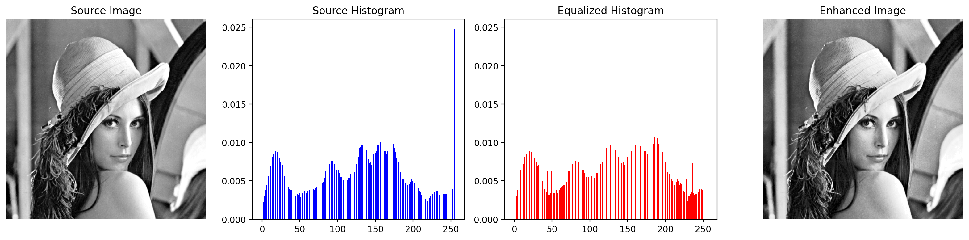
showEqualizedImg(lenna, equalize(lenna))
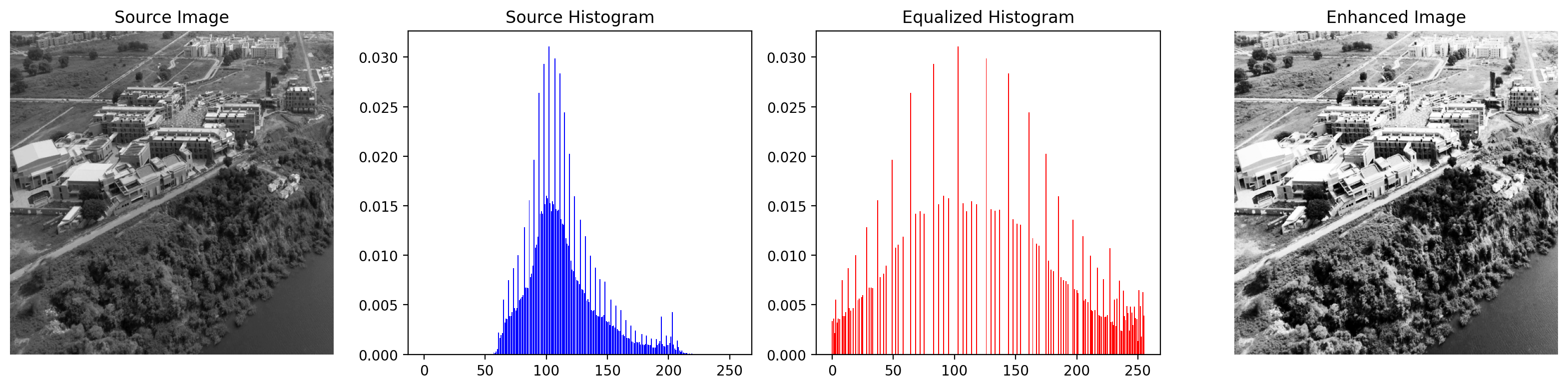
showEqualizedImg(campus, equalize(campus))
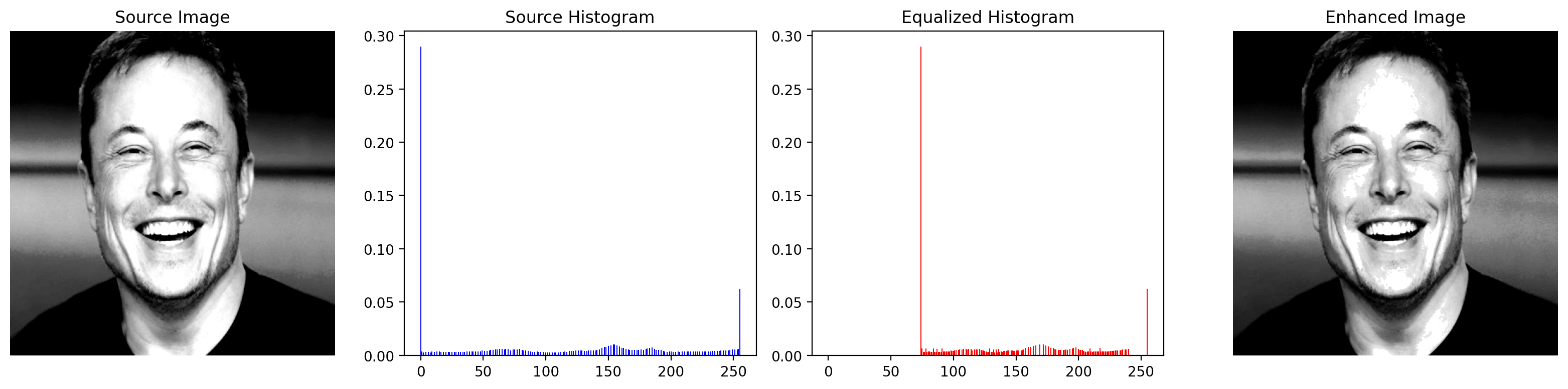
showEqualizedImg(elon, equalize(elon))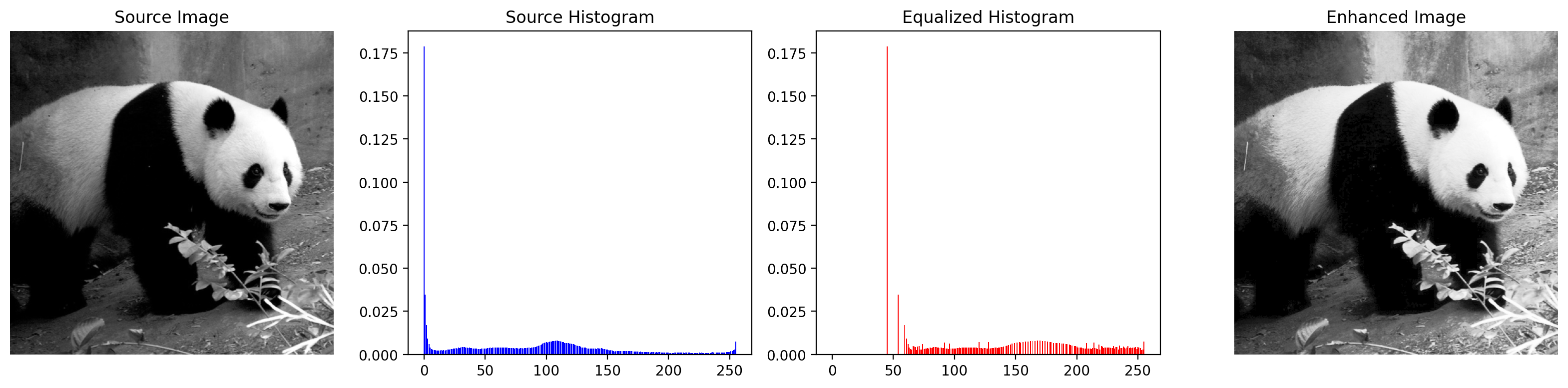

Histogram Matching

Consider a grayscale input image \(X\). It has a probability density function \(p_r(r)\), where \(r\) is a grayscale value, and \(p_r(r)\) is the probability of that value. This probability can easily be computed from the histogram of the image by \[p_r(r_j)=\frac{n_j}{n}\] Where \(n_j\) is the frequency of the grayscale value \(r_j\), and \(n\) is the total number of pixels in the image. Now consider a desired output probability density function \(p_z(z)\). A transformation of \(p_r(r)\) is needed to convert it to \(p_z(z)\). \ Each pdf (probability density function) can be mapped to its cumulative distribution function by \[S(r_k)=\sum\limits_{j=0}^{k}p_r(r_j), \qquad k =0,1,2,...,L-1\] \[G(z_k)=\sum\limits_{j=0}^{k}p_z(z_j), \qquad k =0,1,2,...,L-1\] Where L is the total number of gray levels (here \(L=256\)). \ The idea is to map each \(r\) value in \(X\) to the \(z\) value that has the same probability in the desired pdf: \[S(r_j) = G(z_i) \text{ or } z = G^{-1}(S(r))\]

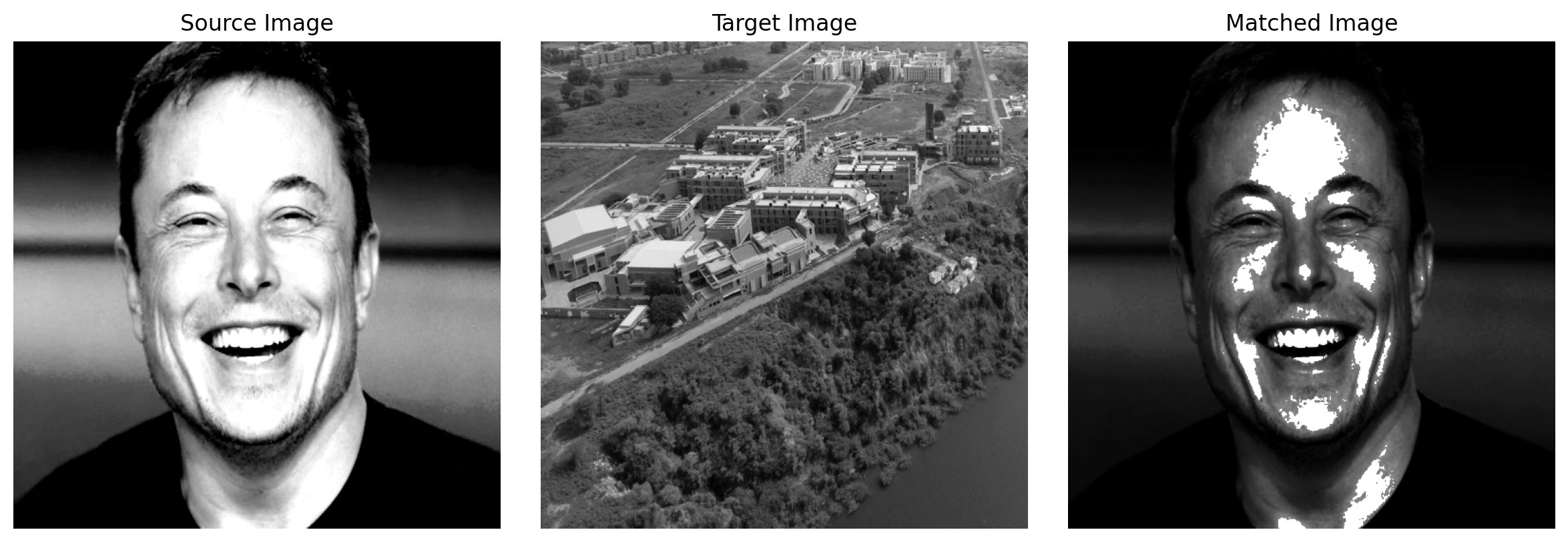
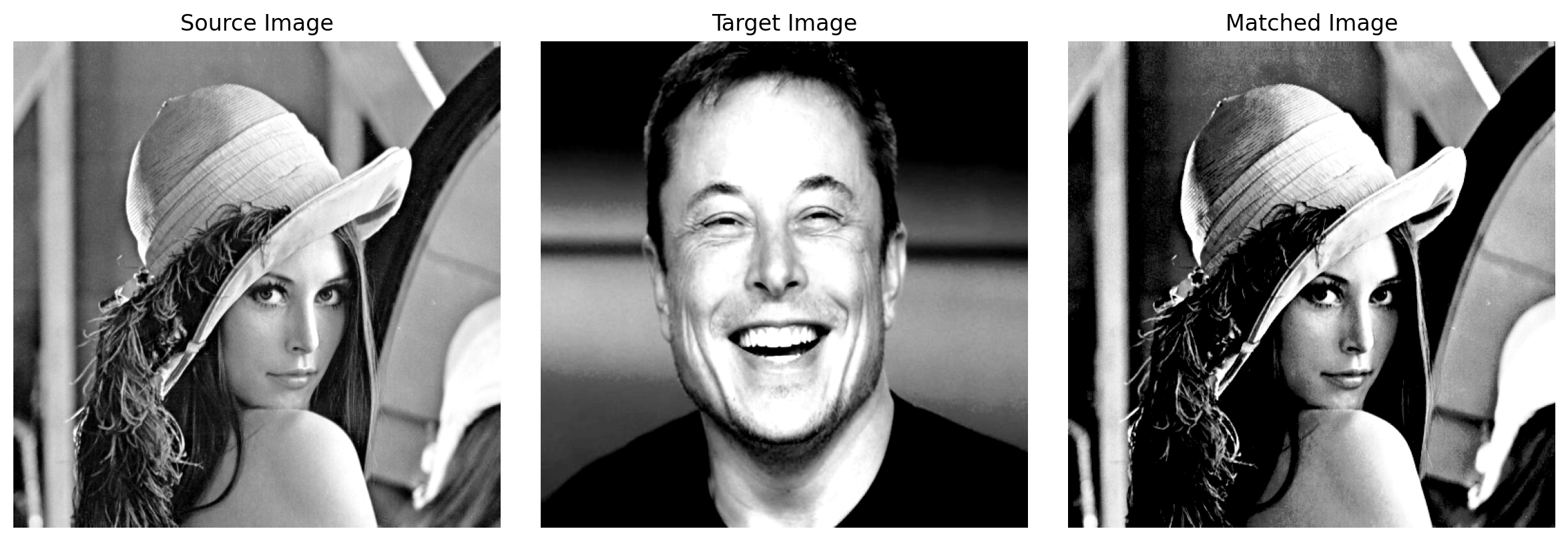
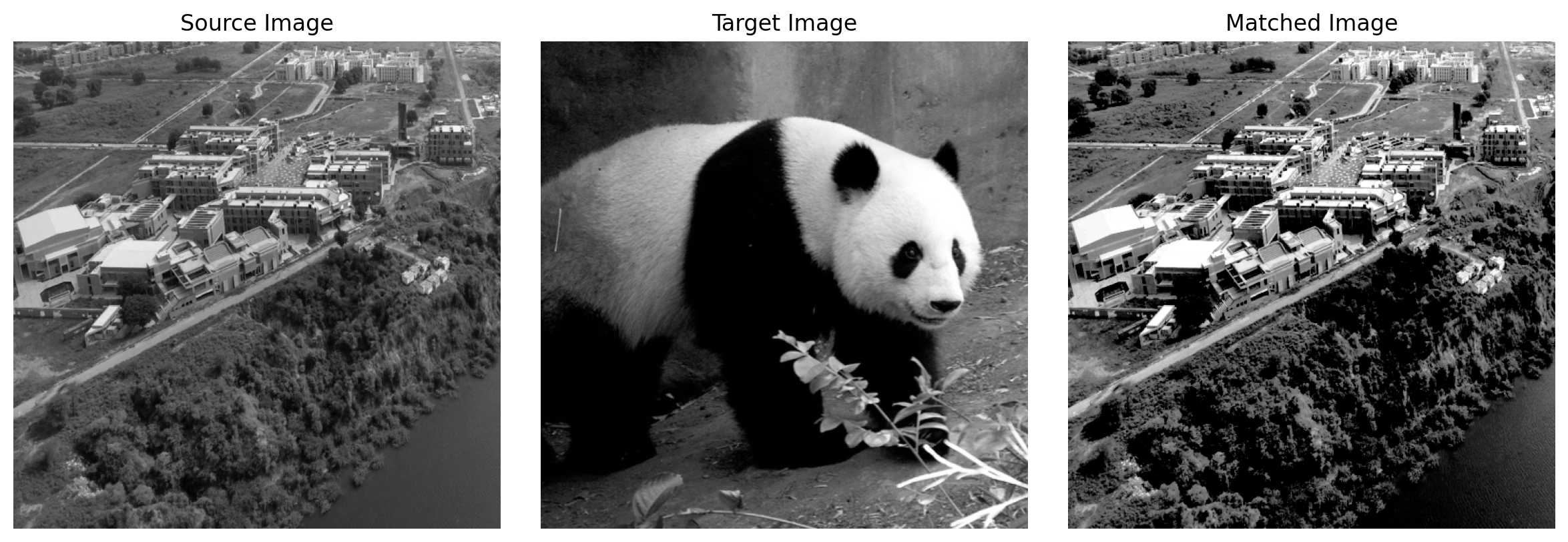
Algorithm \ Given two images, the reference and the target images, we compute their histograms. Following, we calculate the cumulative distribution functions of the two images’ histograms: \(F_1\) for for the reference image and \(F_2\) for the target image. Then for each gray level \(G_1 \in [0, 255]\), we find the gray level \(G_2\) for which \(F_1(G_1)=F_2(G_2)\) and this is the result of histogram matching function: \(M(G_1) = G_2\). Finally, we apply the function \(M\) on each pixel of the reference image.

Code

def match(source_image, target_image):
  source_hist = imgToHist(source_image)
  target_hist = imgToHist(target_image)
  cdf_source_hist = np.cumsum(source_hist) # F1
  cdf_target_hist = np.cumsum(target_hist) # F2
  matched = np.zeros_like(source_image)
  for x_pixel in range(source_image.shape[0]):
    for y_pixel in range(source_image.shape[1]):
      pixel_val = source_image[x_pixel, y_pixel] # G1
      index = 255 # assume G2
      # to find G2
      for i in range(256):
        if cdf_target_hist[i] - cdf_source_hist[pixel_val] >= 0:
          index = i
          break
      # applying function on each pixel
      matched[x_pixel, y_pixel] = index
  return matched

A function is defined to source image, target image and image obtained upon matching. \ cmap is explicity defined to be gray since the default color map is virdis

Code

def showMatchedImg(source_img, target_img, matched_img):
    fig, axes = plt.subplots(1, 3, figsize=(12, 4))
    # source image
    axes[0].imshow(source_img, cmap='gray')
    axes[0].set_title('Source Image')
    axes[0].axis('off')
    # target image
    axes[1].imshow(target_img, cmap='gray')
    axes[1].set_title('Target Image')
    axes[1].axis('off')
    # matched image
    axes[2].imshow(matched_img, cmap='gray')
    axes[2].set_title('Matched Image')
    axes[2].axis('off')

    plt.tight_layout()
    plt.show()

Code

def imageMatch(sourceImage, targetImage):
  matchedImage = match(sourceImage, targetImage)
  showMatchedImg(sourceImage, targetImage, matchedImage)
# according to submission requirements
imageMatch(panda, lenna)
imageMatch(elon, campus)
imageMatch(lenna, elon)
imageMatch(campus, panda)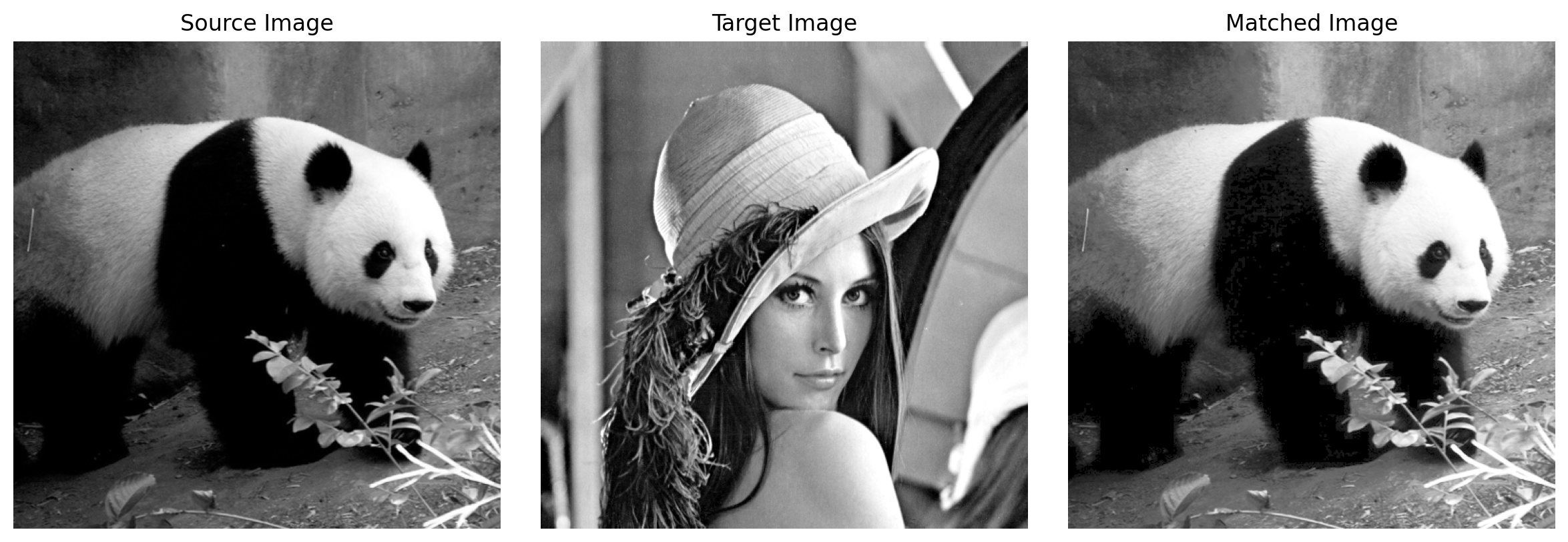

References

[1] Wikipedia Contributors, “Histogram equalization,” Wikipedia, May 18, 2018. https://en.wikipedia.org/wiki/Histogram_equalization

[2] “Histogram matching,” Wikipedia, Feb. 07, 2022. https://en.wikipedia.org/wiki/Histogram_matching