Recurrent Neural Networks from Scratch

The feed-forward networks we’ve built so far are powerful, but they are stateless. They process each input independently, with no memory of what came before. They cannot understand the order in a sentence or the trend in a time series.

Enter Recurrent Neural Networks (RNNs).

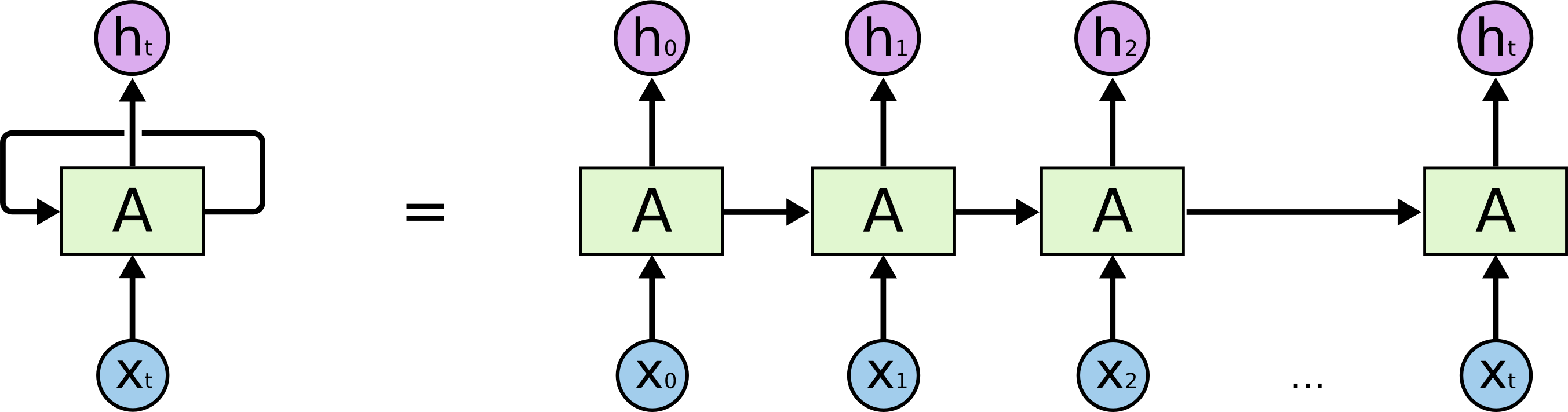
An RNN is a type of neural network designed to handle sequential data. It does this by introducing a loop. At each step in a sequence, the network processes an input and combines it with information from the previous step. This “memory” of the past is stored in a vector called the hidden state.

Credit: Colah’s blog

The core formula that defines a simple RNN is beautifully elegant:

\[ h_t = \tanh(x_t W_{xh} + h_{t-1} W_{hh} + b_h) \]

Where: - \(h_t\) is the new hidden state (the output for the current step). - \(x_t\) is the input vector at the current time step. - \(h_{t-1}\) is the hidden state from the previous step. - \(W_{xh}\), \(W_{hh}\), and \(b_h\) are the learnable weight and bias parameters that are shared across all time steps. This weight sharing is the key that allows the RNN to generalize across sequences of different lengths.

In this post, we will: 1. Implement a simple RecurrentBlock and the tanh activation function from scratch. 2. Build a character-level RNN model. 3. Train it to generate new, unique names based on a list of thousands of examples.

All code for this post can be found in the from_scratch/ directory of the bare-bones-ml repository.

New Library Components

To build our RNN, we only need to add two new pieces to our library.

1. The tanh Activation Function

The hyperbolic tangent (tanh) function is the traditional non-linearity used in simple RNNs. It squashes its input to a range between -1 and 1. Its derivative is simple: \(\frac{d}{dx}\tanh(x) = 1 - \tanh^2(x)\), which is important for backpropagation.

# from_scratch/functional.py

class Tanh(Function):
    def forward(self, x: np.ndarray) -> np.ndarray:
        output = np.tanh(x)
        self.save_for_backward(output)
        return output
    def backward(self, grad: np.ndarray):
        output, = self.saved_tensors
        return grad * (1 - output**2)

def tanh(x: Tensor) -> Tensor:
    return Tanh.apply(x)

2. The RecurrentBlock Module

Our RecurrentBlock will implement a single step of the RNN forward pass. The looping over the sequence will happen explicitly in our training code. This allows us to realize the process of passing the hidden state from one time step to the next, which is often hidden inside a framework’s implementation.

We also make a design choice to combine the weights W_xh and W_hh into a single, larger weight matrix w. We then concatenate the input x and the previous hidden state h_prev to perform a single, efficient matrix multiplication.

# from_scratch/nn.py

class RecurrentBlock(Module):
    """A simple Recurrent Neural Network (RNN) block."""
    def __init__(self, input_size: int, hidden_size: int):
        super().__init__()
        self.hidden_size = hidden_size
        concat_size = input_size + hidden_size
        self.w = Tensor(np.random.randn(concat_size, hidden_size) * 0.01, requires_grad=True)
        self.b_h = Tensor(np.zeros(hidden_size), requires_grad=True)

    def forward(self, x: Tensor, h_prev: Tensor) -> Tensor:
        """Performs one step of the RNN computation."""
        combined = Tensor.cat([x, h_prev], axis=1)
        h_next = tanh(combined @ self.w + self.b_h)
        return h_next

    def parameters(self) -> List[Tensor]:
        return [self.w, self.b_h]

The Task: Character-Level Name Generation

We will train our RNN on a list of thousands of names. The model will learn by reading a name one character at a time and trying to predict the next character in the sequence. For the name “emma”, the training examples would be: - Given a start token ., predict “e”. - Given “e”, predict “m”. - Given “m”, predict “m”. - Given “m”, predict “a”. - Given “a”, predict the end token ..

By training on this task, the model learns the statistical patterns of names: which letters tend to follow others, common prefixes and suffixes, and typical name lengths.

Data Preparation

First, we need to load the data and create our character-level vocabulary. For this task, the “vocabulary” is simply the set of all unique characters present in the dataset, plus a special token (.) to signify the start and end of a name. We will represent each character as a one-hot vector.

import sys
sys.path.append('../')

import numpy as np
import random
from from_scratch.autograd.tensor import Tensor

# 1. The Dataset
# Download from: https://github.com/karpathy/makemore/blob/master/names.txt
# And place it in a `data/` directory at the root of your project.
try:
    with open('../data/names.txt', 'r') as f:
        names = [name.lower() for name in f.read().splitlines()]
except FileNotFoundError:
    print("Error: `data/names.txt` not found.")
    print("Please download it from https://github.com/karpathy/makemore/blob/master/names.txt")
    names = []

if names:
    print(f"Loaded {len(names)} names. First 5: {names[:5]}")

    # 2. Create the Vocabulary
    chars = sorted(list(set("." + "".join(names))))
    char_to_int = {ch: i for i, ch in enumerate(chars)}
    int_to_char = {i: ch for i, ch in enumerate(chars)}
    vocab_size = len(chars)

    print(f"\nVocabulary size: {vocab_size}")
    print(f"Characters: {''.join(chars)}")

    # 3. Helper to create a training example (input sequence and target sequence)
    def get_random_example():
        name = random.choice(names)
        full_sequence = "." + name + "."
        
        input_indices = [char_to_int[c] for c in full_sequence[:-1]]
        target_indices = [char_to_int[c] for c in full_sequence[1:]]
        
        # One-hot encode the input sequence
        input_one_hot = np.zeros((len(input_indices), vocab_size), dtype=np.float32)
        input_one_hot[np.arange(len(input_indices)), input_indices] = 1

        return Tensor(input_one_hot), Tensor(np.array(target_indices))

    # Test the helper
    test_input, test_target = get_random_example()
    print(f"\nExample Input Shape: {test_input.shape}")
    print(f"Example Target Shape: {test_target.shape}")

Loaded 32033 names. First 5: ['emma', 'olivia', 'ava', 'isabella', 'sophia']

Vocabulary size: 27
Characters: .abcdefghijklmnopqrstuvwxyz

Example Input Shape: (6, 27)
Example Target Shape: (6,)

The Model and Training Loop

Our full model will consist of our RecurrentBlock and a Linear output layer. At each time step, the RNN processes a character and updates its hidden state. This hidden state is then passed to the Linear layer to produce logits—raw scores for each character in our vocabulary. We use cross_entropy loss to compare these logits to the true next character.

The key to training an RNN is that the total loss for a sequence is the sum of the losses at each time step. We then call backward() on this final accumulated loss to compute gradients for the entire unrolled sequence. This process is called Backpropagation Through Time (BPTT).

from from_scratch.nn import RecurrentBlock, Linear
from from_scratch.optim import Adam
from from_scratch.functional import cross_entropy

if names:
    # Model Definition
    hidden_size = 128
    rnn_layer = RecurrentBlock(input_size=vocab_size, hidden_size=hidden_size)
    output_layer = Linear(input_size=hidden_size, output_size=vocab_size)

    # Group all parameters for the optimizer
    all_params = rnn_layer.parameters() + output_layer.parameters()
    optimizer = Adam(params=all_params, lr=0.005)

    # Training Loop
    epochs = 20000
    print_every = 1000
    
    print("\n--- Training Start ---")
    for epoch in range(epochs):
        input_tensor, target_tensor = get_random_example()
        
        optimizer.zero_grad()
        
        hidden = Tensor(np.zeros((1, hidden_size)))
        total_loss = Tensor(0.0)
        
        # Explicitly loop through the sequence (BPTT)
        for t in range(input_tensor.shape[0]):
            x_t = input_tensor[t:t+1, :]
            
            # RNN step: Pass input and previous hidden state
            hidden = rnn_layer(x_t, hidden)
            
            # Output layer to get prediction for this step
            logits = output_layer(hidden)
            
            # Calculate loss for this step
            target_t = target_tensor[t:t+1]
            loss = cross_entropy(logits, target_t)
            
            # Accumulate the loss
            total_loss = total_loss + loss

        # Backward pass on the final accumulated loss for the whole sequence
        total_loss.backward()
        
        # Gradient clipping to prevent exploding gradients
        for p in all_params:
            if p.grad is not None:
                np.clip(p.grad, -5, 5, out=p.grad)
                
        optimizer.step()
        
        if epoch % print_every == 0 or epoch == epochs - 1:
            avg_loss = total_loss.data.item() / input_tensor.shape[0]
            print(f"Epoch {epoch}, Avg Loss: {avg_loss:.4f}")

--- Training Start ---
Epoch 0, Avg Loss: 3.2939
Epoch 1000, Avg Loss: 2.2758
Epoch 2000, Avg Loss: 2.2232
Epoch 3000, Avg Loss: 2.0630
Epoch 4000, Avg Loss: 2.4795
Epoch 5000, Avg Loss: 2.5284
Epoch 6000, Avg Loss: 2.7203
Epoch 7000, Avg Loss: 2.6240
Epoch 8000, Avg Loss: 2.6727
Epoch 9000, Avg Loss: 3.1646
Epoch 10000, Avg Loss: 3.0949
Epoch 11000, Avg Loss: 1.9882
Epoch 12000, Avg Loss: 3.0557
Epoch 13000, Avg Loss: 2.3218
Epoch 14000, Avg Loss: 3.1589
Epoch 15000, Avg Loss: 2.4487
Epoch 16000, Avg Loss: 1.7396
Epoch 17000, Avg Loss: 2.7295
Epoch 18000, Avg Loss: 2.9926
Epoch 19000, Avg Loss: 3.1630
Epoch 19999, Avg Loss: 1.9218

Generating New Names

The reward for training a generative model is seeing what it creates! To generate a name, we give the model a starting letter and an initial hidden state of zeros. We then enter a loop: 1. Feed the current character and hidden state to the model to get logits for the next character. 2. Convert the logits to probabilities using softmax. 3. Sample a character from this probability distribution. 4. Feed this new character as the input for the next time step. 5. Repeat until the model generates the special “end” token (.).

from from_scratch.functional import softmax

def generate_name(start_letter='a', max_len=20):
    def char_to_tensor(char):
        tensor = np.zeros((1, vocab_size))
        tensor[0, char_to_int[char]] = 1
        return Tensor(tensor)

    hidden = Tensor(np.zeros((1, hidden_size)))
    current_input = char_to_tensor(start_letter)
    name = start_letter
    
    for _ in range(max_len):
        hidden = rnn_layer(current_input, hidden)
        logits = output_layer(hidden)
        
        probs = softmax(logits)
        
        next_char_idx = np.random.choice(len(chars), p=probs.data.flatten())
        
        if int_to_char[next_char_idx] == '.':
            break
            
        next_char = int_to_char[next_char_idx]
        name += next_char
        current_input = char_to_tensor(next_char)
            
    return name

print("\n--- Generated Names ---")
for char in "abcde":
    print(generate_name(char))

--- Generated Names ---
an
ban
caylsa
deo
el

Conclusion and Next Steps

We have successfully built our first stateful model! It can process inputs of varying lengths and generate new sequences that capture the statistical patterns of the training data.

However, simple RNNs suffer from a major issue: the vanishing gradient problem. As sequences get longer, it becomes very difficult for gradients to flow back to the beginning of the sequence, making it hard for the model to learn long-range dependencies (e.g., how the first letter of a name influences the last).

In our next post, we will tackle this problem by implementing a more advanced and powerful recurrent architecture: the Long Short-Term Memory (LSTM) network.